Due Date
Mon 04/04, 11:59pm
Overview
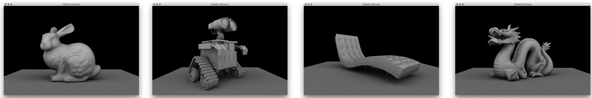
In this project you will implement a simple path tracer that can render pictures with global illumination effects. The first part of the assignment will focus on providing an efficient implementation of ray-scene geometry queries. In the second half of the assignment you will add the ability to simulate how light bounces around the scene, which will allow your renderer to synthesize much higher-quality images. Much like in assignment 2, input scenes are defined in COLLADA files, so you can create your own scenes for your scenes to render using free software like Blender.)
Getting started
We will be distributing assignments with git. You can find the repository for this assignment at http://462cmu.github.io/asst3_pathtracer/. If you are unfamiliar with git, here is what you need to do to get the starter code:
$ git clone https://github.com/462cmu/asst3_pathtracer.git
This will create a asst3_pathtracer folder with all the source files.
Build Instructions
In order to ease the process of running on different platforms, we will be using CMake for our assignments. You will need a CMake installation of version 2.8+ to build the code for this assignment. The GHC 5xxx cluster machines have all the packages required to build the project. It should also be relatively easy to build the assignment and work locally on your OSX or Linux. Building on Windows is currently not supported.
If you are working on OS X and do not have CMake installed, we recommend installing it through Macports:
sudo port install cmake
Or Homebrew:
brew install cmake
To build your code for this assignment:
- Create a directory to build your code:
$ cd asst3_pathtracer && mkdir build && cd build
- Run CMake to generate makefile:
$ cmake ..
- Build your code:
$ make
- (Optionally) install the executable (to asst3_pathtracer/bin):
$ make install
Using the Path Tracer app
When you have successfully built your code, you will get an executable named pathtracer. The pathtracer executable takes exactly one argument from the command line, which is the path of a COLLADA file describing the scene. For example, to load the Keenan cow dae/meshEdit/cow.dae from your build directory:
./pathtracer ../dae/meshEdit/cow.dae
The following are pathtracer app command line options, which are provided for convenience and to debug debugging:
| Commandline Option | Description |
|---|---|
-t <INT> |
Number of threads used for rendering (default=1) |
-s <INT> |
Set the number of camera rays per pixel (default=1) (should be a power of two) |
-l <INT> |
Number of samples to integrate light from area light sources (default=1, higher numbers decrease noise but increase rendering time) |
-m <INT> |
Maximum ray "depth" (the number of bounces on a ray path before the path is terminated) |
-h |
Print command line help |
Mesh Editor Mode
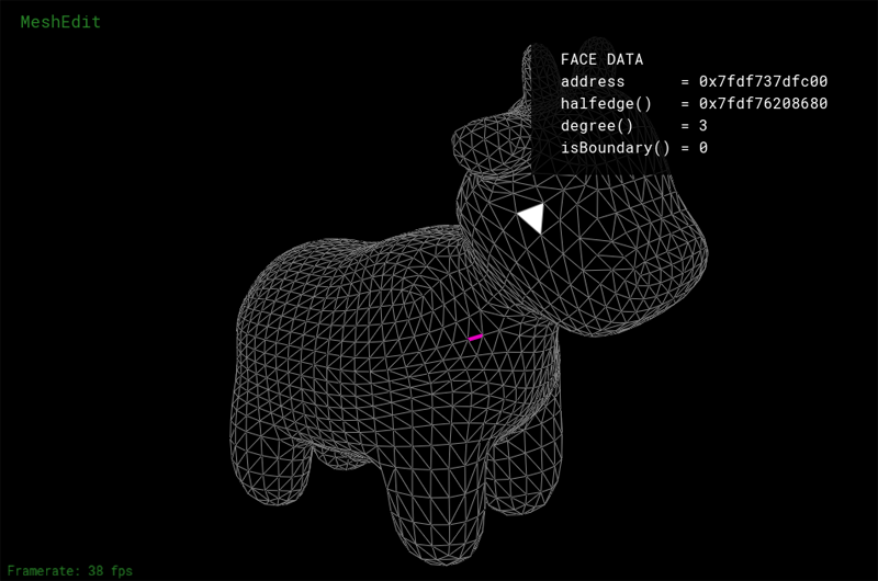
When you first run the application, you will see an interactive wireframe view of the scene that should be familiar to you from Assignment 2. You can rotate the camera by left-clicking and dragging, zoom in/out using the scroll wheel (or multi-touch scrolling on a trackpad), and translate (dolly) the camera using right-click drag. Hitting the spacebar will reset the view.
As with assignment 2, you'll notice that mesh elements (faces, edges, and vertices) under the cursor are highlighted. Clicking on these mesh elements will display information about the element and its associated data. The UI has all the same mesh editing controls as the MeshEdit app from Assignment 2 (listed below). If you want, you can copy your implementation of these operators from Assignment 2 into your Assignment 3 codebase, then you will be able to edit scene geometry using the app.
Rendered Output Mode and BVH Visualization Mode
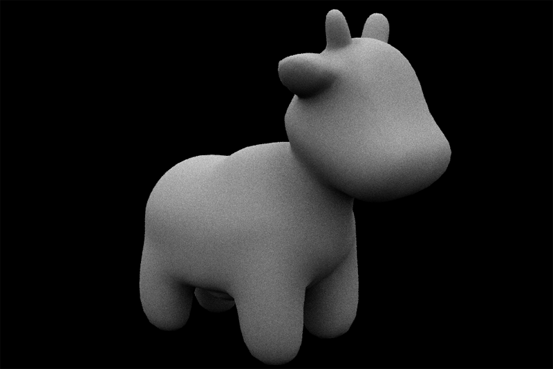
In addition to the mesh editing UI, the app features two other UI modes. Pressing the R key toggles display to the rendered output of your ray tracer. If you press R in the starter code, you will see a black screen (You have not implemented your ray tracer yet! ). However, a correct implementation of the assignment will make pictures of the cow that looks like the one below.
Pressing E returns to the mesh editor view. Pressing V displays the BVH visualizer mode, which will be a helpful visualization tool for debugging the bounding volume hierarchy you will need to implement for this assignment. (More on this later.)
Summary of Viewer Controls
A table of all the keyboard controls in the interactive mesh viewer part of the pathtracer application is provided below.
| Command | Key |
|---|---|
| Flip the selected edge | F |
| Split the selected edge | S |
| Collapse the selected edge | C |
| Upsample the current mesh | U |
| Downsample the current mesh | D |
| Resample the current mesh | M |
| Toggle information overlay | H |
| Return to mesh edit mode | E |
| Show BVH visualizer mode | V |
| Show ray traced output | R |
| Decrease area light samples (RT mode) | - |
| Increase area light samples (RT mode) | + |
| Decrease samples (camera rays) per pixel | [ |
| Increase samples (camera rays) per pixel | ] |
| Descend to left child (BVH viz mode) | LEFT |
| Descend to right child (BVH viz mode) | RIGHT |
| Move to parent node (BVH viz mode) | UP |
| Reset camera to default position | SPACE |
| Edit a vertex position | (left-click and drag on vertex) |
| Rotate camera | (left-click and drag on background) |
| Zoom camera | (mouse wheel) |
| Dolly (translate) camera | (right-click and drag on background) |
Getting Acquainted with the Starter Code
Following the design of modern ray tracing systems, we have chosen to implement the ray tracing components of the Assignment 3 starter code in a very modular fashion. Therefore, unlike previous assignments, your implementation will touch a number of files in the starter code. The main structure of the code base is:
- The main workhorse class is
Pathtracerdefined in pathtracer.cpp. Inside the ray tracer class everything begins with the methodPathtracer::raytrace_pixel()in pathtracer.cpp. This method computes the value of the specified pixel in the output image. - The camera is defined in the
Cameraclass in camera.cpp. You will need to modify `Camera::generate_ray()' in Part 1 of the assignment to generate the camera rays that are sent out into the scene. - Scene objects (e.g., triangles and spheres) are instances of the
Primitiveinterface defined in static_scene/Primitive.h. You will need to implement thePrimitive::intersect()method for both triangles and spheres. - Lights implement the
Lightinterface defined in static_scene/Light.h. The initial starter code has working implementations of directional lights and constant hemispherical lights. - Light energy is represented by instances of the
Spectrumclass. While it's tempting, we encourage you to avoid thinking of spectrums as colors -- think of them as a measurement of energy over many wavelengths. Although our current implementation only represents spectrums by red, green, and blue components (much like the RGB representations of color you've used previously in this class), this abstraction makes it possible to consider other implementations of spectrum in the future. Spectrums can be converted into colors using theSpectrum::toColor()method. - A major portion of the first half of the assignment concerns implementing a bounding volume hierarchy (BVH) that accelerates ray-scene intersection queries. The implementation of the BVH will be located in bvh.cpp/.h. Note that a BVH is also an instance of the
Primitiveinterface (A BVH is a scene primitive that itself contains other primitives.)
Please refer to the inline comments (or the Doxygen documentation) for further details.
Task 1: Generating Camera Rays
"Camera rays" emanate from the camera and measure the amount of scene radiance that reaches a point on the camera's sensor plane. (Given a point on the virtual sensor plane, there is a corresponding camera ray that is traced into the scene.)
Take a look at Pathtracer::raytrace_pixel() in pathtracer.cpp. The job of this function is to compute the amount of energy arriving at this pixel of the image. Conveniently, we've given you a function Pathtracer::trace_ray(r) that provides a measurement of incoming scene radiance along the direction given by ray r.
When the number of samples per pixel is 1, you should sample incoming radiance at the center of each pixel by constructing a ray r that begins at this sensor location and travels through the camera's pinhole. Once you have computed this ray, then call Pathtracer::trace_ray(r) to get the energy deposited in the pixel.
Step 1: Given the width and height of the screen, and point in screen space, compute the corresponding coordinates of the point in normalized ([0-1]x[0x1]) screen space in Pathtracer::raytrace_pixel(). Pass these coordinates to the camera via Camera::generate_ray() in camera.cpp.
Step 2: Implement Camera::generate_ray(). This function should return a ray in world space that reaches the given sensor sample point. We recommend that you compute this ray in camera space (where the camera pinhole is at the origin, the camera is looking down the -Z axis, and +Y is at the top of the screen.) Note that the camera maintains camera-space-to-world space transform c2w that will be handy.
Step 3: Your implementation of Pathtracer::raytrace_pixel() must support supersampling (more than one sample per pixel). The member Pathtracer::ns_aa in the raytracer class gives the number of samples of scene radiance your ray tracer should take per pixel (a.k.a. the number of camera rays per pixel. Note that Pathtracer::gridSampler->get_sample() provides uniformly distributed random 2D points in the [0-1]^2 box (see the implementation in sampler.cpp).
Tips:
Since it'll be hard to know if you camera rays are correct until you implement primitive intersection, we recommend debugging your camera rays by checking what your implementation of
Camera::generate_ray()does with rays at the center of the screen (0.5, 0.5) and at the corners of the image.Before starting to write any code, go through the existing code and make sure you understand the camera model we are using.
Extra credit ideas:
- Modify the implementation of the camera to simulate a camera with a finite aperture (rather than a pinhole camera). This will allow your ray tracer to simulate the effect of defocus blur.
- Write your own
Sampler2Dimplementation that generates samples with improved distribution. Some examples include:- Jittered Sampling
- Multi-jittered sampling
- N-Rooks (Latin Hypercube) sampling
- Sobol sequence sampling
- Halton sequence sampling
- Hammersley sequence sampling
Task 2: Intersecting Triangles and Spheres
Now that your ray tracer generates camera rays, you need to implement ray-primitive intersection routines for the two primitives in the starter code: triangles and spheres. This handout will discuss the requirements of intersecting primitives in terms of triangles.
The Primitive interface contains two types of intersection routines:
bool Triangle::intersect(const Ray& r)returns true/false depending on whether rayrhits the triangle.bool Triangle::intersect(const Ray& r, Intersection *isect)returns true/false depending on whether rayrhits the triangle, but also populates anIntersectionstructure with information describing the surface at the point of the hit.
You will need to implement both of these routines. Correctly doing so requires you to understand the fields in the Ray structure defined in ray.h.
-
Ray.orepresents the 3D point of origin of the ray -
Ray.drepresents the 3D direction of the ray (this direction will be normalized) -
Ray.min_tandRay.max_tcorrespond to the minimum and maximum points on the ray. That is, intersections that lie outside theRay.min_tandRay.max_trange should not be considered valid intersections with the primitive.
There are also two additional fields in the Ray structure that can be helpful in accelerating your intersection computations with bounding boxes (see the BBox class in bbox.h). You may or may not find these precomputed values helpful in your computations.
-
Ray.inv_dis a vector holding (1/x, 1/d.y, 1/d.z) -
Ray.sin[3]hold indicators of the sign of each component of the ray's direction.
One important detail of the Ray structure is that min_t and max_t are mutable fields of the Ray. This means that these fields can be modified by constant member functions such as Triangle::Intersect(). When finding the first intersection of a ray and the scene, you almost certainly want to update the ray's max_t value after finding hits with scene geometry. By bounding the ray as tightly as possible, your ray tracer will be able to avoid unnecessary tests with scene geometry that is known to not be able to result in a closest hit, resulting in higher performance.
Step 1: Intersecting Triangles
While faster implementations are possible, we recommend you implement ray-triangle intersection using the method described in the lecture slides. Further details of implementing this method efficiently are given in these notes.
There are two important details you should be aware of about intersection:
-
When finding the first-hit intersection with a triangle, you need to fill in the
Intersectionstructure with details of the hit. The structure should be initialized with:-
t: the ray's t-value of the hit point -
n: the normal of the surface at the hit point. This normal should be the interpolated normal (obtained via interpolation of the per-vertex normals according to the barycentric coordinates of the hit point) -
primitive: a pointer to the primitive that was hit -
bsdf: a pointer to the surface brdf at the hit point (obtained viamesh->get_bsdf())
-
When intersection occurs with the back-face of a triangle (the side of the triangle opposite the direction of the normal) you should return the normal of triangle pointing away from the side of the triangle that was hit.
If you need to distinguish back-face-hit and front-face-hit in your implementation, you might consider adding a flag(e.g. bool is_back_hit) to the 'Intersection' structure.
Once you've successfully implemented triangle intersection, you will be able to render many of the scenes in the scenes directory ( /dae)). However, your ray tracer will be very slow!
Step 2: Intersecting Spheres
Please also implement the intersection routines for the Sphere class in sphere.cpp. Remember that your intersection tests should respect the ray's min_t and max_t values.
Task 3: Implementing a Bounding Volume Hierarchy (BVH)
In this task you will implement a bounding volume hierarchy that accelerates ray-scene intersection. All of this work will be in the BVHAccel class in bvh.cpp.
The starter code constructs a valid BVH, but it is a trivial BVH with a single node containing all scene primitives. A BVHNode has the following fields:
-
BBox bb: the bounding box of the node (bounds all primitives in the subtree rooted by this node) -
int start: start index of primitives in the BVH's primitive array -
size_t range: range of index in the primitive list (number of primitives in the subtree rooted by the node) -
BVHNode* l: left child node -
BVHNode* r: right child node
The BVHAccel class maintains an array of all primitives in the BVH (primitives). The fields start and range in the BVHNode refer the range of contained primitives in this array.
Step 1: Your job is to construct a BVH using the Surface Area Heuristic discussed in class. Tree construction should occur when the BVHAccel object is constructed.
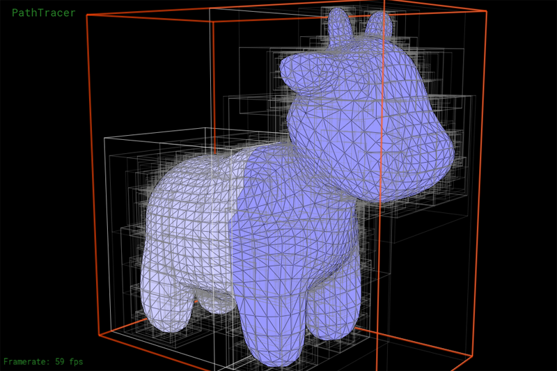
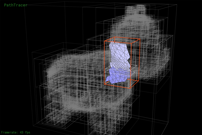
We have implemented a number of tools to help you debug the BVH. Press the V key to enter BVH visualization mode. This mode allows you to directly visualize a BVH as shown below. The current BVH node is highlighted in red. Primitives in the left and right subtrees of the current BVH node are rendered in different colors. Press the LEFT or RIGHT keys to descend to child nodes of the mesh. Press UP to move the parent of the current node.
Another view showing the contents of a lower node in the BVH:
Step 2: Implement the ray-BVH intersection routines required by the Primitive interface. You may wish to consider the node visit order optimizations we discussed in class. Once complete, your renderer should be able to render all of the test scenes in a reasonable amount of time.
Task 4: Implementing Shadow Rays
In this task you will modify Raytracer::trace_ray() to implement accurate shadows.
Currently trace_ray computes the following:
- It computes the intersection of ray
rwith the scene. - It computes the amount of light arriving at the hit point
hit_p(the irradiance at the hit point) by integrating radiance from all scene light sources. - It computes the radiance reflected from the
hit_pin the direction of-r. (The amount of reflected light is based on the brdf of the surface at the hit point.)
Shadows occur when another scene object blocks light emitted from scene light sources towards the hit point (hit_p). Fortunately, determining whether or not a ray of light from a light source to the hit point is occluded by another object is easy given a working ray tracer (which you have at this point!). You simply want to know whether a ray originating from the hit point (p_hit), and traveling towards the light source (dir_to_light) hits any scene geometry before reaching the light (note, the light's distance from the hit point is given by dist_to_light).
Your job is to implement the logic needed to compute whether hit_p is in shadow with respect to the current light source sample. Below are a few tips:
- A common ray tracing pitfall is for the "shadow ray" shot into the scene to accidentally hit the same triangle as
r(the surface is erroneously determined to be occluded because the shadow ray is determined to hit the surface!). We recommend that you make sure the origin of the shadow ray is offset from the surface to avoid these erroneous "self-intersections". For example,o=p_hit + epsilon * dir_to_light(note:EPS_Dis defined for this purpose). - You will find it useful to debug your shadow code using the
DirectionalLightsince it produces hard shadows that are easy to reason about.
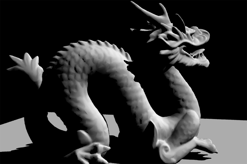
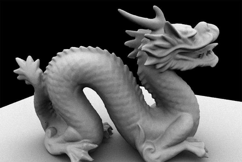
At this point you should be able to render very striking images. For example, here is the Stanford Dragon model rendered with both a directional light and a hemispherical light.
Task 5: Adding Path Tracing
A few notes before getting started:
The new release of the starter code for tasks 5-7 makes a few changes and improvements to the original starter code of the assignment:
The
BRDFclass has been renamedBSDF(for "bidirectional scattering distribution function") to indicate that the class is now responsible for computing both light that is reflected from the surface, but also light that is refracted as it is transmitted through the surface. Implementations reside in bsdf.cpp/h.Rather than use a single hardcoded light source in your
Pathtracer::trace_ray()lights are now defined as part of the scene description file.
You should change your implementation of the reflectance estimate due to direct lighting in Pathtracer::trace_ray() to iterate over the list of scene light sources using the following code:
for (SceneLight* light : scene->lights) {
    /// do work here...
}
-
PathTracer::raytrace_pixel(size_t x, size_t y)now returns aSpectrumfor the pixel (it doesn't directly update the output image). The update is now handled inPathTracer::raytrace_tile()and is included in the starter code.
In this task you will modify your ray tracer to add support for indirect illumination. We wish for you to implement the path tracing algorithm that terminates ray paths using Russian Roulette, as discussed in class. Recommend that you restructure the code in Pathtracer::trace_ray() as follows:
Pathtracer::trace_ray() {
  if (surface hit) {
       //
       // compute reflectance due to direct lighting only
       //
       for each light:
          accumulate reflectance contribution due to light

       //
       // add reflectance due to indirect illumination
       //
       randomly select a new ray direction (it may be
       reflection or transmittence ray depending on
       surface type -- see BSDF::sample_f()

       potentially kill path (using Russian roulette)

       evaluate weighted reflectance contribution due
       to light from this direction
  }
}
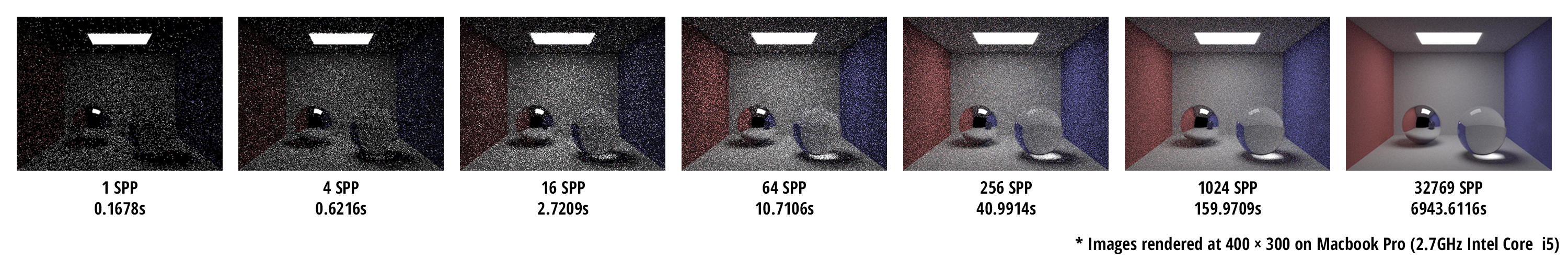
As a warmup for the next task, implement BSDF::sample_f for diffuse surfaces (DiffuseBSDF:sample_f). The implementation of DiffuseBSDF::f is already provided to you. After correctly implementing diffuse BSDF and path tracing, your renderer should be able to make a beautifully lit picture of the Cornell Box with:
./pathtracer -s 1024 -m 2 -t 8 ../dae/sky/CBspheres_lambertian.dae
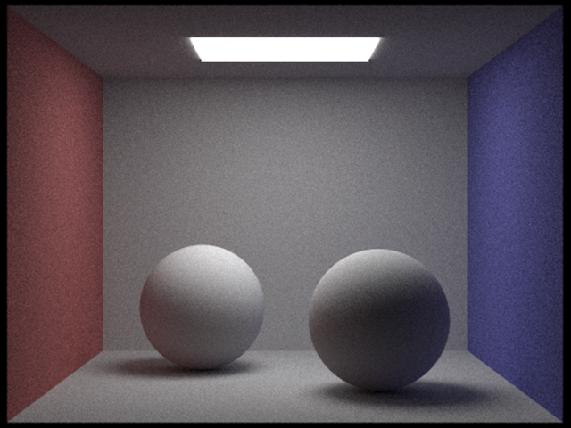
Note the time-quality tradeoff here. With these commandline arguments, your path tracer will be running with 8 worker threads at a sample rate of 256 camera rays per pixel, with a max ray depth of 4. This will produce an image with relatively high quality but will take quite some time to render. Rendering a high quality image will take a very long time as indicated by the image sequence below, so start testing your path tracer early!
Here are a few tips:
The termination probability of paths can be determined based on the overall throughput of the path (you'll likely need to add a field to the
Raystructure to implement this) or based on the value of the BSDF givenwoandwiin the current step. Keep in mind that delta function BRDFs can take on values greater than one, so clamping termination probabilities derived from BRDF values to 1 is wise.To convert a
Spectrumto a termination probability, we recommend you use the luminance (overall brightness) of the Spectrum, which is available viaSpectrum::illum()We've given you some pretty good notes on how to do this part of the assignment, but it can still be tricky to get correct.
Task 6: Adding New Materials
Now that you have implemented the ability to sample more complex light paths, it's finally time to add support for more types of materials (other than the fully Lambertian material provided to you in the starter code). In this task you will add support for two types of materials: a perfect mirror and glass (a material featuring both specular reflection and transmittance).
To get started take a look at the BSDF interface in bsdf.cpp. There are a number of key methods you should understand:
-
BSDF::f(wo,wi)evaluates the distribution function for a given pair of directions. -
BSDF::sample_f(const Vector3D& wo, Vector3D* wi, float* pdf)generates a random samplewo(which may be a reflection direction or a refracted transmitted light direction). The method returns the value of the distribution function for the pair of directions, and the pdf for the selected samplewi.
There are also two helper functions in the BSDF class that you will need to implement:
BSDF::reflect(w0, ...)returns a directionwithat is the perfect specular reflection direction corresponding towi(reflection of w0 about the normal, which in the surface coordinate space is [0,0,1]). More detail about specular reflection is here.BSDF::refract(w0, ...)returns the ray that results from refracting the rayw0about the surface according to Snell's Law. The surface's index of refraction is given by the argumentior. Your implementation should assume that if the rayw0is entering the surface (that is, ifcos(w0,N) > 0) then the ray is currently in vacuum (index of refraction = 1.0). Ifcos(w0,N) < 0then your code should assume the ray is leaving the surface and entering vacuum. In the case of total internal reflection, the method should returnfalse.
What you need to do:
Implement the class
MirrorBSDFwhich represents a material with perfect specular reflection (a perfect mirror). You should ImplementMirrorBSDF::f(),MirrorBSFD::sample_f(), andBSDF::reflect(). (Hint: what should the pdf computed byMirrorBSFD::sample_f()be? What should the reflectance function f() be?)-
Implement the class
GlassBSDFwhich is a glass-like material that both reflects light and transmit light. As discussed in class the fraction of light that is reflected and transmitted through glass is given by the dielectric Fresnel equations, which are documented in detail here. Specifically your implementation should:-
Implement BSDF::refract()to add support for refracted ray paths. - Use the Fresnel equations to compute the fraction of reflected light and the fraction of transmitted light. Your implementation of
- Implement
GlassBSDF::sample_f(). Your implementation should use the Fresnel equations to compute the fraction of reflected light and the fraction of transmitted light. The returned ray sample should be either a reflection ray or a refracted ray, with the probability of which type of ray to use for the current path proportional to the Fresnel reflectance. (e.g., If the Fresnel reflectance is 0.9, then you should generate a reflection ray 90% of the time. What should the pdf be in this case?) - You should read the provided notes on the Fresnel equations as well as on how to compute a transmittance BRDF.
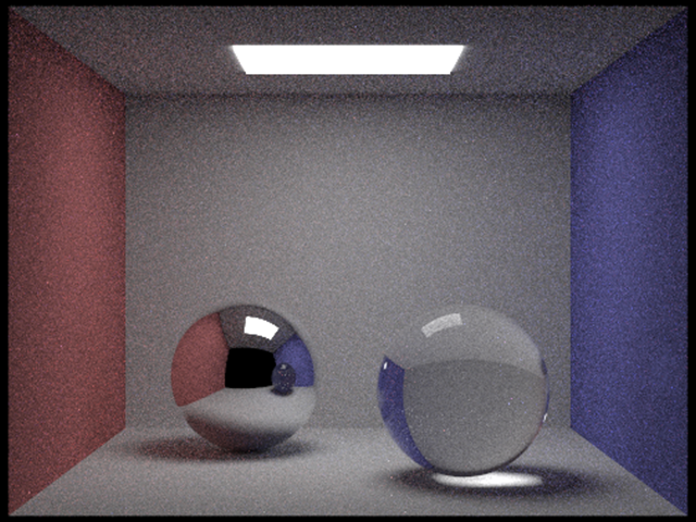
-
When you are done, you will be able to render images like these:
Task 7: Infinite Environment Lighting
The final task of this assignment will be to implement a new type of light source: an infinite environment light. An environment light is a light that supplies incident radiance (really, the light intensity dPhi/dOmega) from all directions on the sphere. The source is thought to be "infinitely far away", and is representative of realistic lighting environments in the real world: as a result, rendering using environment lighting can be quite striking.
The intensity of incoming light from each direction is defined by a texture map parameterized by phi and theta, as shown below.
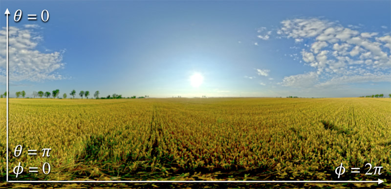
In this task you need to implement the EnvironmentLight::sample_L() method in static_scene/environment_light.cpp. You'll start with uniform direction sampling to get things working, and then move to a more advanced implementation that uses importance sampling to significantly reduce variance in rendered images.
Step one: uniform sampling
To get things working, your first implementation of EnvironmentLight::sample_L() will be quite simple. You should generate a random direction on the sphere (with uniform (1/4pi) probability with respect to solid angle), convert this direction to coordinates (phi, theta) and then look up the appropriate radiance value in the texture map using bilinear interpolation (note: we recommend you begin with bilinear interpolation to keep things simple.)
You an designate rendering to use a particular environment map using the -e commandline parameter: (e.g., -e ../exr/grace.exr )
Since high dynamic range environment maps can be large files, we have not included them in the starter code repo. You can download a set of environment maps from this link.
Tips:
- You must write your own code to uniformly sample the sphere.
-
envMap->datacontains the pixels of the environment map - The size of the environment texture is given by
envMap->wandenvMap->h.
Step two: importance sampling the environment map
Much like light in the real world, most of the energy provided by an environment light source is concentrated in the directions toward bright light sources. Therefore, it makes sense to bias selection of sampled directions towards the directions for which incoming radiance is the greatest. In this final task you will implement an importance sampling scheme for environment lights. For environment lights with large variation in incoming light intensities, good importance sampling will significantly improve the quality of renderings.
The basic idea is that you will assign a probability to each pixel in the environment map based on the total flux passing through the solid angle it represents. We've written up a detailed set of notes for you here (see "Task 7 notes").
Here are a few tips:
- When computing areas corresponding to a pixel, use the value of theta at the pixel centers.
- We recommend precomputing the joint distributions p(phi, theta) and marginal distributions p(theta) in the constructor of
EnvironmentLightand storing the resulting values in fields of the class. -
Spectrum::illum()returns the luminance (brightness) of a Spectrum. The probability of a pixel should be proportional to the product of its luminance and the solid angle it subtends. -
std::binary_searchis your friend. Documentation is here.
Grading
Your code must run on the GHC 5xxxx cluster machines as we will grade on those machines. Do not wait until the submission deadline to test your code on the cluster machines. Keep in mind that there is no perfect way to run on arbitrary platforms. If you experience trouble building on your computer, while the staff may be able to help, but the GHC 5xxx machines will always work and we recommend you work on them.
The assignment consists of a total of 100 pts. The point breakdown is as follows:
- Task 1: 5
- Task 2: 15
- Task 3: 20
- Task 4: 10
- Task 5: 15
- Task 6: 20
- Task 7: 15
Handin Instructions
Your handin directory is on AFS under:
/afs/cs/academic/class/15462-s16-users/ANDREWID/asst3/, or
/afs/cs/academic/class/15662-s16-users/ANDREWID/asst3/
You will need to create the asst3 directory yourself. All your files should be placed there. Please make sure you have a directory and are able to write to it well before the deadline; we are not responsible if you wait until 10 minutes before the deadline and run into trouble. Also, you may need to run aklog cs.cmu.edu after you login in order to read from/write to your submission directory.
You should submit all files needed to build your project, this include:
-
srcfolder with all your source files -
imgfolder with screenshots of CBspheres, CBspheres_lambertian you rendered -
READMEfile
Note: You can save your rendered images from the application by pressing S when your path tracer is done rendering. The screenshots you submit should be rendered at relatively high quality configurations. Feel free to include additional images you have rendered with your path tracer, especially the ones that demonstrates the extra credit features you have implemented.
You should also include, in your README file, the pathtracer configuration you used to render the images are submitting. If you have implemented any of the extra credit features, clearly indicate which extra credit features you have implemented. You should also briefly state anything that you think the grader should be aware of.
Please do not include:
- The
buildfolder - Executables
- Any additional binary or intermediate files generated in the build process
Do not add levels of indirection when submitting. And please use the same arrangement as the handout. We will enter your handin directory, and run:
mkdir build && cd build && cmake .. && make
and your code should build correctly. The code must compile and run on the GHC 5xxx cluster machines. Be sure to check to make sure you submit all files and that your code builds correctly.
Friendly advice from your TAs
As always, start early. There is a lot to implement in this assignment, and no official checkpoint, so don't fall behind! Depending on your implementation, the rendering process might take several hours to finish. So start early to make sure you have enough time to render some beautiful images (which is the most enjoyable part of this assignment).
While C has many pitfalls, C++ introduces even more wonderful ways to shoot yourself in the foot. It is generally wise to stay away from as many features as possible, and make sure you fully understand the features you do use. The C++ Super-FAQ is a great resource that explains things in a way that's detailed yet easy to understand (unlike a lot of C++ resources), and was co-written by Bjarne Stroustrup, the creator of C++!