Due Date
Tue Nov 24th, 11:59pm
Overview
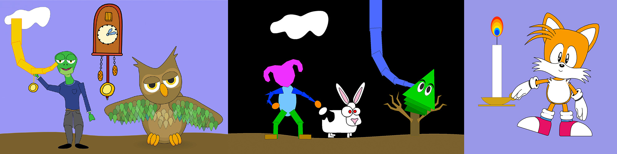
In this project you will build on your previous work with 2D rasterization to implement an application that allows you to manipulate and animate jointed cartoon characters. When you are done, you will have a tool that allows you to produce animations that use three of the major techniques used in production computer animation: keyframing, numerical optimization, and physically-based simulation. (You can create your own SVG characters in free software like Inkscape, or commercial software like Adobe Illustrator; more details are given below about exactly how to construct one of these characters.)
Supplementary Notes
In addition to the writeup on this webpage, you may find the following supplementary material useful in implementing and/or understanding this assignment:
- Reparameterizing a Catmull-Rom Spline - this note shows how to adjust derivative data when using an existing cubic polynomial interpolant on the unit interval [0,1] to implement Catmull-Rom interpolation.
- Derivation of our simple Inverse Kinematics (IK) Algorithm - this note shows how we came up with our simple inverse kinematics scheme, namely: (i) what is our description of a character, (ii) what is the energy we want to minimize, (iii) and how do we take its gradient?
- Equations of Motion for a Translating Compound Pendulum - this note shows how we derived the equations of motion used by your integrator below, and also provides a solution to Quiz 19.
Getting started
We will be distributing assignments with git. You can find the repository for this assignment at https://github.com/462cmu/asst4_animation/. If you are unfamiliar with git, here is what you need to do to get the starter code:
$ git clone https://github.com/462cmu/asst4_animation.git
This will create a asst4_animator folder with all the source files.
Build Instructions
In order to ease the process of running on different platforms, we will be using CMake for our assignments. You will need a CMake installation of version 2.8+ to build the code for this assignment. The GHC 5xxx cluster machines have all the packages required to build the project. It should also be relatively easy to build the assignment and work locally on your OSX or Linux. Building on Windows is currently not supported.
If you are working on OS X and do not have CMake installed, we recommend installing it through Macports:
sudo port install cmake
Or Homebrew:
brew install cmake
To build your code for this assignment:
- Create a directory to build your code:
$ cd asst4_animator && mkdir build && cd build
- Run CMake to generate makefile:
$ cmake ..
- Build your code:
$ make
- Install the executable (to asst4_animator/bin):
$ make install
Using the Animator App
When you have successfully built your code, you will get an executable named animator. The animator executable takes exactly one argument from the command line, specifying either a single SVG character, or a directory containing multiple characters. (Every SVG file in the directory must follow the character format, described below.) For example, to load the example file scenes/character.svg from your build directory:
./meshedit ../scenes/character.svg
Likewise, to load the directory scenes/testscene/ you can run
./meshedit ../scenes/testscene
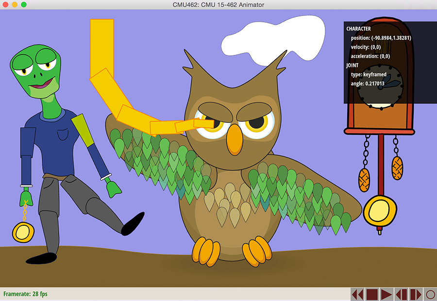
When you first run the application, you will see a collection of one or more characters, possibly overlapping. As you move the cursor around the screen, you'll notice that the character joint under the cursor gets highlighted. Clicking on this joint will display its attributes and current state. As you implement more features, you will be able to manipulate the character by clicking and dragging on its joints.
In this assignment, you will add functionality to the program that allows you to give motion to the characters in a variety of ways. There will be three basic types of animation:
- Keyframed - At each point in time, the user can set the joint angles and translation for each of the characters. These events are inserted into a spline data structure, that interpolates the values over time. Your task will be to implement the interpolation routines, which return the interpolated value and its derivatives.
- Inverse Kinematics (IK) - Setting every joint in a character is difficult and time consuming. In the second part of the assignment you will implement a simple inverse kinematics scheme that allows the character configuration to be modified by dragging a point on the character toward a target point. Your key tasks will be computing the gradient of the IK energy, and implementing a simple gradient descent scheme to update the joint angles.
- Dynamics - Some of the characters have special "pendulum" joints whose motion will be dictated by physically-based simulation rather than keyframe interpolation. Your job will be to evaluate the forces and integrate the equations of motion for a swinging pendulum. Note that the axis of rotation for this pendulum may be driven by the motion of a keyframed joint; these additional forces also need to be accounted for in the dynamics so that, for instance, an image tossed around the scene will exhibit lively dynamics.
The user interface for each of these animation modes is described in the table below. Notice that currently, nothing happens when the scene is animated - this is because you haven't yet implemented any of these modes of animation! Unlike the previous assignment, no reference solution is provided. However, we provide visual debugging feedback that should help determine if your solutions are correct. We will also provide several examples (images and video) of correct interpolation, IK, and dynamics.
Summary of Viewer Controls
A table of all the mouse and keyboard controls in the animator application is provided below.
| Command | Key |
|---|---|
| Rotate a joint | (left click and drag on joint) |
| Move a character | (left click and drag on root joint) |
| Manipulate a joint via IK | (right click and drag on a joint) |
| Delete current keyframe | BACKSPACE/DELETE |
| Show/hide debugging information | d |
| Save animation to image sequence | s |
| Play the animation | SPACE |
| Step timeline forward by one frame | RIGHT KEY |
| Step timeline forward by ten frames | RIGHT KEY + SHIFT |
| Step timeline back by one frame | LEFT KEY |
| Step timeline back by ten frames | LEFT KEY + SHIFT |
| Move to next keyframe in timeline | RIGHT KEY + ALT |
| Move to next keyframe in timeline | LEFT KEY + ALT |
| Move to beginning of timeline | UP KEY/HOME |
| Move to end of timeline | DOWN KEY/END |
| Make timeline shorter | [ |
| Make timeline shorter | ] |
The timeline can also be manipulated by clicking on the timeline itself. Clicking and dragging will "scrub" through the animation; clicking on the buttons will play, pause, loop, etc.
What You Need to Do
The assignment is divided into three parts:
- Keyframe animation
- Inverse kinematics
- Dynamics simulation
As with all of our assignments, this assignment involves significant implementation effort. Also, be advised that there are some dependencies, e.g., IK and dynamics both depend on properly-working keyframe interpolation. Therefore, you are highly advised to compete the interpolation tasks first, and to carefully consider the correctness of this code, since it will be used by subsequent tasks.
Getting Acquainted with the Starter Code
Before you start, here are some basic information on the structure of the starter code.
Your work will be constrained to implementing part of the classes Spline, Joint, and Character in spline.h and character.cpp. The routines you need to implement will be clearly marked at the top of the file. You should be able to implement all the necessary routines without adding additional members or methods to the classes. You can also assume that a character has already been correctly loaded and built from an SVG file; you do not have to worry about malformed input. (Of course, if you create your own malformed SVG files, you might run into trouble!)
The Character and Joint classes
The main object you will be working with is a Character, which is a tree-like collection of Joints together with some additional information, such as its position as a function of time. Each Joint is a node in the tree, which stores pointers to all of its children plus additional information encoding its center of rotation, and rotation angle as a function of time (relative to the parent). Each joint also has a flag specifying whether its motion should be determined by keyframe interpolation, or by dynamics.
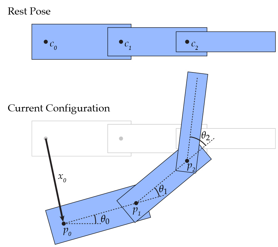
When working with characters, it is very important to understand how its state (positions, rotation centers, and angles) encodes its configuration. In particular, let $x_0(t)$ denote the translation of the character as a function of time, encoded by the member Character::position. Let $c_i$ denote the fixed center of rotation for joint $i$, encoded by the member Character::center (note that this value is not the geometric center of the object; it is an arbitrary point that could be anywhere on the object--or even somewhere off the object!). Finally, let $\theta_i(t)$ denote the angle of rotation for joint i as a function of time, encoded by either the member Character::angle (for keyframe interpolated joints), or Character::theta (for dynamic joints). At any given time $t$, the rotation of joints and translation of characters will move each joint center to a new location $p_i$, which we will ultimately store in the member Character::currentCenter. If joint $j$ is the parent of joint $i$, then the current position of the root can be expressed as
$$p_0 = c_0 + x_0(t)$$
and the current position of any (non-root) node $i$ can be expressed as
$$p_i = p_j + R(\Theta_i(t)) ( c_i - c_j )$$
where $R(s)$ denotes a counter-clockwise rotation by the angle $s$ (in radians), and $\Theta_i(t)$ denotes the cumulative rotation from the root node all the way down to joint $i$ (at time $t$). In other words, to get the position of any joint, we start at the parent joint, and add the difference between the two joints' centers, rotated by all of the angles "above" the current joint. The cumulative rotation can be written explicitly as
$$\Theta_i(t) = \sum_{k=0}^{i-1} \theta_k(t)$$
Consider what happens, for instance, when the root translation and all the angles are zero. Then we have $p_0$ = $c_0$, and hence
$$p_1 = p_0 + R(0) ( c_1 - c_0 ) = c_0 + c_1 - c_0 = c_1$$
$$p_2 = p_1 + R(0) ( c_2 - c_1 ) = c_1 + c_2 - c_1 = c_2$$
and so forth. In other words, we just recover the original joint centers.
In your code, you will not compute these cumulative rotations explicitly, but rather by recursively traversing the tree. I.e., each joint will compute its transformation relative to its parent, and then pass this updated transformation to all of its children so that they can compute their own transformations. This kind of hierarchical scene graph is typical in many computer graphics applications (both 2D and 3D).
The Character and Joint classes have some additional members that will help you to compute their motion. For instance, each joint stores its current transformation and the current transformation of its parent; it also stores values to encode the current angle and angular velocity for dynamical simulation. You should take a close look at the comments in the header file character.h to get a more detailed understanding of how these classes work.
IMPORTANT As in many computer graphics applications, the convention used for our coordinate system is that the vertical axis points down, not up! In mathematics, the vertical axis typically points up. When you were writing your rasterizer, this wasn't such a big deal: at worst, the picture shows up inverted, which you immediately realize and fix. With dynamics, having the wrong coordinate system can cause all sorts of trouble! Make sure you understand what coordinate systems you are working with (especially when it comes to things like rotation). Otherwise, you can get some pretty funny behavior.
Task 1: Keyframe Interpolation
As we discussed in class, data points in time can be interpolated by constructing an approximating piecewise polynomial or spline. In this assignment you will implement a particular kind of spline, called a Catmull-Rom spline. A Catmull-Rom spline is a piecewise cubic spline defined purely in terms of the points it interpolates. It is a popular choice in real animation systems, because the animator does not need to define additional data like tangents, etc. (However, your code may still need to numerically evaluate these tangents after the fact; more on this point later.) All of the methods relevant to spline interpolation can be found in spline.h with implementations in spline.inl.
Task 1A: Hermite curve over the unit interval
Recall that a cubic polynomial is a function of the form
$$p(t) = at^3 + bt^2 + ct + d$$
where $a, b, c$, and $d$ are fixed coefficients. However, there are many different ways of specifying a cubic polynomial. In particular, rather than specifying the coefficients directly, we can specify the endpoints and tangents we wish to interpolate. This construction is called the "Hermite form" of the polynomial. In particular, the Hermite form is given by
$$p(t) = h_{00}(t)p_0 + h_{10}(t)m_0 + h_{01}(t)p_1 + h_{11}(t)m_1$$
where $p_0,p_1$ are the endpoint positions, m0,m1 are the endpoint tangents, and hij are the Hermite bases
$$h_{00}(t) = 2t^3 - 3t^2 + 1$$
$$h_{10}(t) = t^3 - 2t^2 + t$$
$$h_{01}(t) = -2t^3 + 3t^2$$
$$h_{11}(t) = t^3 - t^2$$
Your first task is to implement the method Spline::cubicSplineUnitInterval(), which evaluates a spline defined over the time interval $[0,1]$ given a pair of endpoints and tangents at endpoints. Optionally, the user can also specify that they want one of the time derivatives of the spline (1st or 2nd derivative), which will be needed for our dynamics calculations.
Your basic strategy for implementing this routine should be:
Evaluate the time, its square, and its cube. (For readability, you may want to make a local copy of
normalizedTimecalled simplyt.)Using these values, as well as the position and tangent values, compute the four basis functions $h_{00}, h_{01}, h_{10},$ and $h_{11}$ of a cubic polynomial in Hermite form. Or, if the user has requested the nth derivative, evaluate the nth derivative of each of the bases.
Finally, combine the endpoint and tangent data using the evaluated bases, and return the result.
Notice that this function is templated on a type T. In C++, a templated class can operate on data of a variable type. In the case of a spline, for instance, we want to be able to interpolate all sorts of data: angles, vectors, colors, etc. So it wouldn't make sense to rewrite our spline class once for each of these types; instead, we use templates. In terms of implementation, your code will look no different than if you were operating on a basic type (e.g., doubles). However, the compiler will complain if you try to interpolate a type for which interpolation doesn't make sense! For instance, if you tried to interpolate Character objects, the compiler would likely complain that there is no definition for the sum of two characters (via a + operator). In general, our spline interpolation will only make sense for data that comes from a vector space, since we need to add T values and take scalar multiples.
Task 1B: Evaluation of a Catmull-Rom spline
Using the routine from part 1A, you will now implement the method Spline::evaluate() which evaluates a general Catmull-Rom spline (and possibly one of its derivatives) at the specified time. Since we now know how to interpolate a pair of endpoints and tangents, the only task remaining is to find the interval closest to the query time, and evaluate its endpoints and tangents.
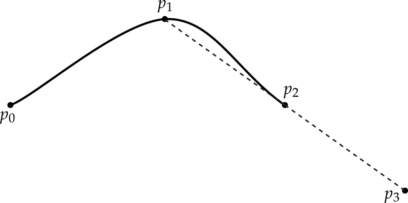
The basic idea behind Catmull-Rom is that for a given time t, we first find the four closest knots at times
$$t_0 < t_1 \leq t < t_2 < t_3$$
We then use t1 and t2 as the endpoints of our cubic "piece," and for tangents we use the values
$$m_1 = ( p_2 - p_0 ) / (t_2 - t_0)$$
$$m_2 = ( p_3 - p_1 ) / (t_3 - t_1)$$
In other words, a reasonable guess for the tangent is given by the difference between neighboring points. (See the Wikipedia and our course slides for more details.)
This scheme works great if we have two well-defined knots on either side of the query time t. But what happens if we get a query time near the beginning or end of the spline? Or what if the spline contains fewer than four knots? We still have to somehow come up with a reasonable definition for the positions and tangents of the curve at these times. For this assignment, your Catmull-Rom spline interpolation should satisfy the following properties:
If there are no knots at all in the spline, interpolation should return the default value for the interpolated type. This value can be computed by simply calling the constructor for the type:
T(). For instance, if the spline is interpolatingVector2Dobjects, then the default value will be $(0,0)$.If there is only one knot in the spline, interpolation should always return the value of that knot (independent of the time). In other words, we simply have a constant interpolant. (What, therefore, should we return for the 1st and 2nd derivatives?)
- If the query time is less than or equal to the initial knot, return the initial knot's value. (What do derivatives look like in this region?)
- If the query time is greater than or equal to the final knot, return the final knot's value. (What do derivatives look like in this region?)
Once we have two or more knots, interpolation can be handled using general-purpose code; we no longer have to consider individual cases (two knots, three knots, ...). In particular, we can adopt the following "mirroring" strategy:
- Any query time between the first and last knot will have at least one knot "to the left" $(k_1)$ and one "to the right" $(k_2)$.
- Suppose we don't have a knot "two to the left" $(k_0)$. Then we will define a "virtual" knot $k_0 = k_1 - (k_2-k_1)$. In other words, we will "mirror" the difference be observe between $k_1$ and $k_2$ to the other side of $k_1$.
- Likewise, if we don't have a knot "two to the left" of $t (k_3)$, then we will "mirror" the difference to get a "virtual" knot $k_3 = k_2 + (k_2-k_1)$.
- At this point, we have four valid knot values (whether "real" or "virtual"), and can compute our tangents and positions as usual.
- These values are then handed off to our subroutine that computes cubic interpolation over the unit interval.
An important thing to keep in mind is that Spline::cubicSplineUnitInterval() assumes that the time value t is between 0 and 1, whereas the distance between two knots on our Catmull-Rom spline can be arbitrary. Therefore, when calling this subroutine you will have to normalize t such that it is between 0 and 1, i.e., you will have to divide by the length of the current interval over which you are interpolating. You should think very carefully about how this normalization affects the value and derivatives computed by the subroutine, in comparison to the values and derivatives we want to return.
Internally, a Spline object stores its data in an STL map that maps knot times to knot values. A nice thing about an STL map is that it automatically keeps knots in sorted order. Therefore, we can quickly access the knot closest to a given time using the method map::upper_bound(), which returns an iterator to knot with the smallest time greater than the given query time (you can find out more about this method via online documentation for the Standard Template Library).
Trying it out
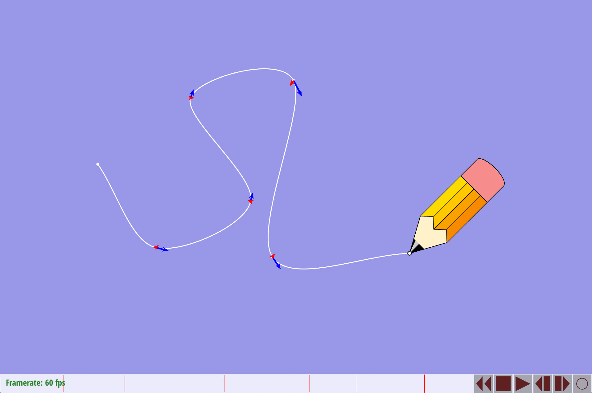
As soon as spline animation is working, you should be able to edit and playback animations in the timeline. The first thing you should try is translating a character along a spline path by dragging the root node of the character to different locations in the scene at different points in time (the root node is usually something like the character's torso). (A good example is pencil.svg.) If position interpolation is working properly, you should see a white curve interpolating the points of translation. If derivative interpolation is working, you should also see blue arrows visualizing the velocity, and red arrows visualizing the acceleration. Compare with the example below.
Now make something fun!
Possible Extra Credit Extensions:
- There are a variety of variants on the Catmull-Rom spline that are used in computer animation such as the Centripetal Catmull-Rom spline. Find and implement different types of spline interpolation that are well-suited to our 2D keyframe animation, and provide some justification for why they should improve the motion or the ease of generating an animation. Produce animations that demonstrate the pros and cons of the different interpolation schemes. (Another interesting example are the so-called wiggly splines.)
Task 2: Inverse Kinematics
After playing with spline interpolation a bit, you may have noticed that it takes a lot of work to manipulate characters into the desired pose, especially if they have many joints (check out character.svg, for instance). In this task you will implement a basic inverse kinematics (IK) solver that optimizes joint angles in order to meet a given target. In particular, it will try to match a selected point on the character to the current position of the cursor.
Above, we already described how positions in our kinematic chain are determined from the current angles $\theta_i$. Our IK algorithm will try to adjust these angles so that our character "reaches for" the cursor. In particular, suppose the user clicks on a point p on joint $i$, then moves the cursor to a point $q$ on the screen. We want to minimize the objective
$$f_0(\theta) = | p(\theta) - q |^2$$
with respect to the joint angles theta. To keep things simple, we're going to adopt the following convention:
The source position p is expressed with respect to the original coordinate system of the joint, i.e., before its parent character translation and joint rotations are applied.
This way, $p(\theta)$ is the position of the source point after transformation by theta (and the character center). For instance, if $p$ were the joint center, then $p(\theta)$ would just be equal to $p_i(\theta)$, i.e., the transformed joint center.
Task 2A: Evaluate the gradient
The question now is: what is the derivative of $f_0$ with respect to one of the angles $\theta_j$? Of course, we only have to consider angles $\theta_j$ "further up the chain" from joint $i$, because angles below joint $i$ (or angles on other branches of the tree) don't affect the position of the transformed source point. Suppose, then, that joint $j$ is an ancestor of joint $i$. Then the derivative of $f_0$ with respect to $\theta_j$ is given by
$$< q-p(\theta), u >$$
where <.,.> denotes the usual dot product and u is the vector
$$R(\pi/2)( p(\theta) - p_j(\theta) )$$
i.e., we take the difference between the current source point and the current location of the jth joint, rotated by 90 degrees.
This formula will be evaluated in the method Joint::calculateAngleGradient() found in the 'character.h' file. This method takes three parameters:
- a pointer to the joint $i$ that contains the source point,
- the current position $p(\theta)$ of the source point (i.e., the transformed click point), and
- the current position $q$ of the target point (i.e., the mouse cursor).
It should compute the gradient of $f_0$ with respect to joint's angle and store it in the member Joint::ikAngleGradient. It should also recursively evaluate the gradient for all children, i.e., it should call calculateAngleGradient() for each of the "kids." However, you should be sure not to set an angle gradient for any joint that doesn't affect the source point; the angle gradient for all other joints must be set to zero. To aid in this process, you can use the boolean return value of Joint::calculateAngleGradient() to help determine whether the current branch is connected to the joint containing the source point.
One thing to think about is: do you want the root joint to rotate? For instance, if we are trying to manipulate the hand of a character, should the entire body rotate to meet the goal? In practice, this can lead to some annoying/counter-intuitive behavior, and in practice we might like the character to remaining "sitting upright." Therefore, in the reference implementation (and the examples below) we set the IK gradient for the root node to zero. At least for the purposes of debugging your implementation, you should also set Joint::ikAngleGradient to zero for the root node, which you can easily do (for instance) in the method Character::reachForTarget(), which has explicit knowledge of the root node via the member Character::root.
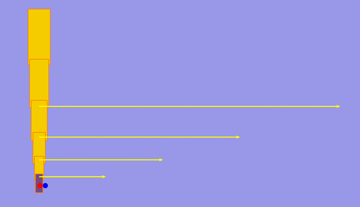
Once you have implemented this method, you will be able to see a visualization of the angle gradients by right-clicking and dragging on a joint. For instance, if you load up the example file scenes/testscene/telescope.svg, your implementation should match the gradients visualized below; here the red dot is the initial click point, and the blue dot is the position of the cursor. However, the configuration of the character should not change (yet).
IMPORTANT Please note that you will first need to call the Joint::calculateAngleGradient() method in the Character::reachForTarget() method in your code before any visual outputs will be present. To match the picture below, you should make sure to set gradientLengthScale to $0.1$ in the method Animator::drawIKDebugWidgets(), which can be found in animator.cpp.
Task 2B: Ski downhill
From here, there's not much more to do: we simply need to "ski downhill" (i.e., apply gradient descent) using the gradient we computed in part 2B. In particular, you will need to implement the method Character::reachForTarget(), which takes three parameters:
- a pointer to the joint containing the click point,
- the location of the un-transformed source point (i.e., without the character translation or joint rotations applied),
- the target point (i.e., the location of the cursor), and
- the current animation time.
This method will need to do several things:
- First, it needs to call
update(), which computes the current configuration of each joint. (These values are used by your gradient subroutine, therefore they need to be updated for the current animation time.) - Also, it needs to compute the angle gradient for every joint. Joints that do not influence the objective should have zero gradient. IMPORTANTLY you must transform the source point into its current configuration before passing it to
Joint::calculateGradient(); the joint's current transformation is stored in the memberJoint::currentTransformation. - Finally, it needs to advance the joint angles via gradient descent. This can be done by iterating over all joints and adding a little bit of the angle derivative to the current angle (forward Euler).
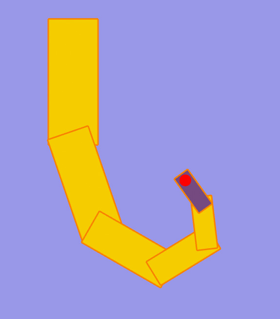
How do you pick the size of the time step? For this assignment, we will just use a "very small" time step (the reference implementation uses a time step of $\tau = 0.000001$, but feel free to experiment). Also, to get snappier feedback, you can take multiple gradient descent steps per call to Character::reachForTarget() (we used 10... but please experiment so you get a sense of how this all works!). When things are working properly, the telescope should bend as in the picture below. (Now try generating some animation, using your new IK tool to accelerate the process!)
Possible Extra Credit Extensions:
As noted above, we pick our gradient descent time step in an extremely naive way: just a small constant that remains the same independent of what kind of character we're animating, and how big our displacements are. In general, picking a fixed time step for gradient descent is a recipe for disaster! Implement a more intelligent line search strategy that takes the value of the objective and the gradient into account when picking the time step. Simple but effective strategies include backtracking line search, Armijo-Wolfe, and golden section search.
In class, we also discussed the fact that first-order methods like gradient descent can be extremely slow to converge whenever the energy landscape looks like a "long slender valley." Implement a second-order descent strategy to speed up convergence of your IK solver. Note, however, that since the objective is nonconvex, naive Newton descent will not work (why?). Instead, you will likely want to use a quasi-Newton method; one that is very popular in graphics (and quite effective in practice) is L-BFGS, which can be nicely computed using only the function values and gradients (i.e., no Hessian is needed). Likewise, the Gauss-Newton method requires only the gradient values, and is well suited to objectives that are sums of squares (like our IK "closeness" objective).
Incorporate limits on the joint angles (which are often found in real systems like robots, and are also convenient for character animation). These joint angles become simple linear inequality constraints in the optimization problem, and are fairly easy to handle via the projected gradient method.
The IK algorithm you've implemented in this assignment is only one of many possible methods (closely related to the "Jacobian transpose" method)—other possibilities include "Jacobian inverse" and "cyclic coordinate descent", as well as "Forward and Backward Reaching IK (FABRIK)". Implement one of these methods (or any other IK method) and compare and contrast with our simple gradient descent scheme. What are the advantages and disadvantages of each method? Which methods are best suited to our 2D animation problem? What new kinds of animation might you enable by incorporating different IK schemes?
Task 3: Secondary Dynamics
In the final part of your assignment, you will add additional "secondary" motion to your animations, coming from physically-based dynamics. In particular, you will implement support for special joints whose motion is determined by the dynamics of a swinging pendulum. This motion can be used to animate things like a swinging pendulum on a clock, or cartoony motion for things like feathers on a bird, scales on a lizard, leaves on a tree, and other little pieces of flair (get creative!). The nice thing about physically-based motion is that it comes at "no extra cost" in the sense that an animator using our system will gets additional richness and complexity without specifying anything beyond the existing keyframe animation. However, it will take additional work on your part to implement the dynamics (and additional computational work at run time to perform the numerical integration).
Task 3A: A basic swinging pendulum
To get us started, we will implement a basic swinging pendulum that does not respond to the acceleration of the character it is attached to. To do so, we simply need to implement the equations of motion for a compound pendulum (i.e., a pendulum consisting of a single rigid body rotating around some axis):
$$d^2 \theta/dt^2 = -m \cdot g \cdot L \cdot sin(\theta) / I$$
Here theta is the angle with the vertical, m is the mass, g is the acceleration due to gravity, L is distance between the axis of rotation and the center of mass, and I is the moment of inertia. As we also discussed in class, this second-order (in time) ODE can be split into a system of two first-order ODEs:
$$d \theta / dt = \omega$$
$$d \omega / dt = -m \cdot g \cdot L \cdot sin(\theta) / I$$
It is these equations you will integrate numerically. In our code framework, the angle theta is stored as the member Joint::theta, and the angular velocity omega is stored as the member Joint::omega. You will need to implement the method Joint::integrate(), which takes three parameters:
- the curent time,
- the time step requested by the user, and
- the cumulative acceleration of any joints "above" the current joint.
For this task you should only need the second parameter (i.e., the time step). In particular, you should integrate the equations of motion using the symplectic Euler method, which yields good energy behavior (no blowup or damping) and does not require the use of temporary variables.
The physical attributes $m, L,$ and $I$ of the pendulum can be computed using the method Joint::physicalQuantities(), which will return the mass, moment of inertia, and center of mass (these properties are computed from the shape of the joint as described by the SVG file; you can take a look at the file svg.cpp if you're interested in how they're computed). The length $L$ is the distance between the joint center $c$ and the center of mass $C$, i.e.,
$$L = | C - c |$$
When computing this quantity, you should be careful to use the un-transformed joint center Joint::center rather than the transformed center Joint::currentCenter, since the center of mass $C$ is also expressed in pre-transformed coordinates. For the gravitational acceleration $g$ you can use any constant that gives reasonable animation; the scales of objects in our SVG files (being cartoons) do not relate to any typical physical scale. The reference implementation uses the value $g = 3$.
The only remaining thing you have to do to get your dynamics working is to call your integration routine starting at the root of the character. This can be done by implementing the method Character::integrate(), which should call integrate() on the member root. Note that Joint::integrate() asks for three parameters: the current time, the integration time step, and the body acceleration. For the time being you can just pass in a zero vector for the acceleration; this vector will be worked out in Task 3B.
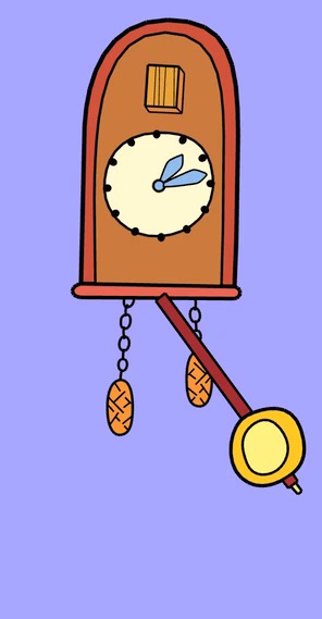
Once everything has been implemented, try animating the pendulum in clock.svg. It should swing back and forth indefinitely, without ever blowing up or dying down. Click here for an example movie.
In the real world, objects do eventually stop moving due to friction and other dissipative forces. The nice thing about starting with an integrator that preserves energy is that it gives us precise control over exactly how much energy is lost each time step. In particular, suppose we take a time step of size $\tau$. Then we can damp our angular velocity $omega$ by simply multiplying it by $exp( -a \tau )$, where a is a positive constant; in the reference implementation we just use $a=1$. (By the way, why is this the damping factor? Well, if the instantaneous damping factor were $a$, then the ODE describing the damping would be the simple linear equation $du/dt = -au$, whose solution is $u(t) = exp( -at ) u(0)$.) After damping, your clock pendulum should gradually slow down; click here for an example movie.
Task 3B:
The integrator implemented in part 3A gives some dynamics to your pendulum, but are still incorrect in two noticeable ways:
- The center of mass is not properly accounted for, meaning that objects that are heavier "on one side" will not hang correctly.
- The pendulum does not react to the motion of the object it is attached to. In this task, you will modify your integrator to account for these two features.
First, consider the equation of motion you implemented in 3A:
$$d \omega / dt = -m \cdot g \cdot L \cdot sin(\theta) / I$$
Here, theta represents the angle with the vertical, but this angle is measured relative to the arbitrary starting configuration of the shapes defined in the SVG file. Instead, we want theta to represent the angle that the center of mass makes with the vertical. As before, the center of mass C can be obtained via the method Joint::physicalQuantities. To adjust your equations of motion, you should:
- Compute the vector y from the center of rotation to the center of mass, in the initial (un-rotated) configuration.
- Compute the angle psi made by the vector y with the vertical. To make sure you get the right angle, independent of what quadrant y is in, you should take a look at the
atan2function from the standard library. (Make sure you are calculating the angle with the vertical, and not the angle with the horizontal!) - Subtract psi from theta in your equations of motion.
Now, when you load a character with pendulums attached to it (like clock.svg) you should see a very slight motion at the beginning of the animation.
Your final task is to adjust the equations of motion so that each pendulum reacts to the motion of objects above it in the character hierarchy. In your quiz, you determined the equations of motion for a moving pendulum; here we will adjust those equations slightly so that the "swinging" motion accounts for the specific shape and size of the pendulum. In particular, you will now want to integrate
$$d \omega / dt = -( < a, y^{perp} > / L^2 + m \cdot g \cdot L \cdot sin(\theta-\psi) / I )$$
where $a$ is the acceleration of the center of rotation of the joint, and $y^{perp}$ is the vector from the center of rotation to the center of mass, rotated by 90 degrees in the counter-clockwise direction.
The only challenge here is computing the acceleration a. This acceleration is the sum of the accelerations due to:
- translation of the root node, and
- rotation of any joint above this joint.
The first part, translation, is easy: you just need to modify Character::integrate() to compute the acceleration due to translation, rather than using the zero vector. If you implemented your spline class correctly, you should be able to call this value by making the appropriate call to position::evaluate(). At this point, you should also pass the current value of time from Character::integrate() to Joint::integrate(), since joints further down the chain may need to know the time in order to evaluate the acceleration of a keyframed joint at the current time.
Next, you will need to modify Joint::integrate() to add any acceleration due to rotation. Notice that acceleration really is additive: for instance if a character is running and its arm is swinging, the total acceleration is the sum of the linear acceleration due to translation plus the linear acceleration due to rotation.
So, how do you compute the linear acceleration due to rotation? Well, consider a joint $m$ and let $n$ be one of its immediate children; recall that $c_m$ and $c_n$ denote the positions of the joint centers prior to any rotation or translation. Let $\alpha$ be the spline-interpolated angle of joint $m$ at the current time, obtained by calling Spline::evaluate() on the member Joint::angle(). Then at the current time we can write the location of the child relative to the parent as a vector
$$ z(t) = R(alpha(t))( c_n - c_m ), $$
where $R(alpha(t))$ denotes a rotation by $alpha(t)$. (Note that this vector will be different for each child!) The first derivative of $z$ with respect to $t$ is the velocity of the center of mass; the second derivative of $z$ with respect to t is its acceleration. You should take these derivatives yourself (i.e., by hand, before writing any more code), being sure to properly apply both the chain rule and the product rule. Remember that you can obtain the first and second derivative of the angle alpha itself by passing the values 1 and 2 as arguments to Spline::evalute(). (As a hint, your final expression should involve both the first and second time derivatives of the angle alpha!)
At this point, you have an expression for the second time derivative of $z$ in the original (un-rotated) coordinate frame. To get the correct acceleration, you will need to rotate this vector by the rotation of the parent transformation Joint::currentParentTransformation. The easiest way to do this is to convert your acceleration vector into homogeneous coordinates setting the third homogeneous component to zero rather than one. By setting the third component to zero, you are effectively saying "apply rotations, but not translations" (since the "translation" column of the homogeneous transform matrix will have no effect on the result; if this doesn't make sense to you, try multiplying the 3x3 homogeneous transform matrix out by hand for a vector with a homogeneous coordinate of 1, and homogeneous coordinate 0). Map the transformed coordinate back to ordinary (2D) coordinates. (Do you need to do a homogeneous divide here? Why or why not?) Finally, pass the sum of the cumulative acceleration and the acceleration due to rotation to the current child. This value will ultimately be used by any "dynamic" joint.
In summary, the steps you need to perform in this task are:
- Adjust your equations of motion to account for the center of mass.
- Initialize the cumulative acceleration using the acceleration of the character position in
Character::integrate(). - Derive an expression for the linear acceleration of the center of mass due to joint rotation in the local coordinate frame.
- In
Joint::integrate(), evaluate the linear acceleration due to rotation in the local coordinate frame. - Transform the acceleration computed in step (3) into the current coordinate frame using
Joint::currentParentTransformation. - Add this transformed acceleration to the cumulative acceleration.
- Pass the cumulative acceleration (and the current time) to all children.
Note that you should add the acceleration due to rotation only if the joint is a keyframed joint; otherwise, you would be using the acceleration of a spline that is not actually used to animate the character! In other words, you should check the joint type Joint::type before adding the acceleration due to keyframed rotation, making sure that its value is KEYFRAMED. (In principle, of course, you should also be accumulating the acceleration due to rotation for any joint, including those whose dynamics are dictated by pendulum motion. Unfortunately, the equations for a double, triple, and n-pendulum get much trickier, since they are no longer uni-directional, i.e., the motion of a joint "further down the chain" also affects the motion of joints "further up the chain." You can attack the problem of multiple pendulums for extra credit, if you so desire.)
Once you have finished implementing this task, the pendulums in your scene should react to character translation and rotation. Click here for an example movie.
Note that the physical quantities computed by Joint::physicalQuantities() do not necessarily correspond to any physically meaningful values (e.g., meters, kilograms, etc.)---they simply arise from the size of objects in the input SVG file. Therefore, in order to get plausible motion, you may need to tweak various constants in your integrator (even in slightly non-physical ways). In the reference implementation, we made the following adjustments for this task:
- The acceleration due to gravity is now set to $g=5000$.
- The length $L$ is divided by 1000 before being used for anything.
- The acceleration due to joint rotation is scaled by $10000$.
You are free to play with these constants in order to make your animation more appealing. Ideally, of course, you would be able to find one set of parameters that is both physically consistent and also leads to attractive motion. However, even in real-world animation systems there is a lot of tweaking of constants. Why is that? For one thing, the objects we're animating are not physical! (Cartoon frogs, etc.) For another thing, getting all the physical parameters correct can be challenging. (Though perhaps still something to strive for as you head out into the world! I.e., can you make an animation system that is both beautiful and physically correct? This point of view has certainly paid off in the world of rendering.)
Possible Extra Credit Extensions:
Allow double, triple, or n-pendulums by correctly integrating their equations of motion. Can you find a clever way to handle a system like this, without grinding out long equations by hand?
Implement a new kind of joint based on a spring potential rather than a pendulum. (How will you then draw the character? One idea is to stretch the joints along the axis of the spring.) Can you combine springs and pendulums? How do you get the right equations of motion?
Our final equations of motion are still not 100% physical in the sense that the acceleration term does not properly account for the shape and size of the joint (i.e., it does not use the moment of inertia, mass, etc.). Derive the full equations of motion for a compound pendulum plus translation of the center of rotation. (This calculation is rather involved, and will require a solid knowledge of vector calculus; in particular, Green's theorem.) Compare animations made using the original and corrected equations of motion. Is there a noticeable difference?
Incorporate constraints on joint angles. How should a pendulum behave if it reaches the limiting angle? Should it "bounce" back in the opposite direction? Perhaps you should use a coefficient of restitution to determine how much energy gets absorbed during the bounce.
Task 4: Get Creative!
Now that you have an awesome animation system, make an awesome animation! You can save your animation to an image sequence by hitting 's' in the viewer, and compress it into a movie using the script in the p4 directory. In "getting creative," you should also try creating your own characters, either using a program like Inkscape or by just creating your own SVG file by hand (see below for more details). Have fun!
Grading
Your code must run on the GHC 5xxxx cluster machines as we will grade on those machines. Do not wait until the submission deadline to test your code on the cluster machines. Keep in mind that there is no perfect way to run on arbitrary platforms. If you experience trouble building on your computer, while the staff may be able to help, but the GHC 5xxx machines will always work and we recommend you work on them.
Each task will be graded on the basis of correctness, except for Task 7 which will be graded (gently) on effort. You are not expected to completely reproduce the reference solution vertex-for-vertex as slight differences in implementation strategy or even the order of floating point arithmetic will causes differences, but your solution should not be very far off from the provided input/output pairs. If you have any questions about whether your implementation is "sufficiently correct", just ask.
The assignment consists of a total of 100 pts. The point breakdown is as follows:
- Task 1A: 12
- Task 1B: 13
- Task 2A: 13
- Task 2B: 12
- Task 3A: 13
- Task 3B: 12
- Task 4: 25
Handin Instructions
Your handin directory is on AFS under:
/afs/cs/academic/class/15462-f15-users/ANDREWID/asst4/
Note that you may need to create the asst4 directory yourself. All your files should be placed there. Please make sure you have a directory and are able to write to it well before the deadline; we are not responsible if you wait until 10 minutes before the deadline and run into trouble. Also, you may need to run aklog cs.cmu.edu after you login in order to read from/write to your submission directory.
You should submit all files needed to build your project, this include:
- The
srcfolder with all your source files
Please do not include:
- The
buildfolder - Executables
- Any additional binary or intermediate files generated in the build process.
You should include a README file (plaintext or pdf) if you have implemented any of the extra credit features. In your REAME file, clearly indicate which extra credit features you have implemented. You should also briefly state anything that you think the grader should be aware of.
Do not add levels of indirection when submitting. And please use the same arrangement as the handout. We will enter your handin directory, and run:
mkdir build && cd build && cmake .. && make
and your code should build correctly. The code must compile and run on the GHC 5xxx cluster machines. Be sure to check to make sure you submit all files and that your code builds correctly.
Friendly Advice from your TAs
As always, start early. There is a lot to implement in this assignment, and no official checkpoint, so don't fall behind!
Be careful with memory allocation, as too many or too frequent heap allocations will severely degrade performance.
Make sure you have a submission directory that you can write to as soon as possible. Notify course staff if this is not the case.
While C has many pitfalls, C++ introduces even more wonderful ways to shoot yourself in the foot. It is generally wise to stay away from as many features as possible, and make sure you fully understand the features you do use.
Rigged Character Definitions
Specially-constructed SVG files are used to define used to describe a kinematic chain that is a hierarchical representation of a character. The grouping and layering of objects is used to determine the hierarchy and dynamic behavior of the character. In particular:
A shape is an elementary SVG shape; currently-supported shapes include: circle, ellipse, rectangle, line segment, polyline, and polygon.
Each joint consists of a single group of shapes, where the last shape in the group must be a circle. This list must be "flat," i.e., it cannot be a group of groups. The circle specifies the center of rotation for the joint (its radius is ignored). The fill color of the joint determines its motion type: black for keyframed joints, white for dynamic joints.
A character is a collection of hierarchically grouped joints. The grouping determines a dependency tree among joints; in particular, in any group of joints the first joint is the parent, and all remaining joints are children. All joints in a file must ultimately be grouped into a single character; there is no support for multiple characters in a single file.
Example: Suppose we want to create a character consisting of a shoulder A, an arm B, a hand C, and three fingers x, y, and z. Each of A, B, C, x, y, and z must be joints, i.e., they must each be a flat list of shapes, including a circle at the very end specifying the center of rotation. For instance, one of the fingers might look like a = (ellipse,ellipse,ellipse,circle), consisting of three finger joints and an axis of rotation. In this case, the three finger joints would be fixed relative to each other; only the whole finger would be able to rotate. To construct the character, we would then construct the group (x,y,z,C), which attaches the five fingers to the hand C. We would then put this group into a group ((x,y,z,C),B) attaching the hand to the arm, and finally (((x,y,z,C),B),A) attaching the arm to the shoulder. Here is the corresponding SVG code; note that comments (beginning with !--) are ignored:
<svg>
   <g> <!-- CHARACTER: jointed arm with fingers -->
      <g> <!-- SHAPE: shoulder (C) -->
         <ellipse cx="40" cy="340" rx="40" ry="50"/>
         <circle cx="40" cy="380" r="1" fill="#000000" /> <!-- center of rotation -->
      </g>
      <g>
         <g> <!-- SHAPE: arm (B) -->
            <rect x="0" y="140" width="80" height="200"/>
            <circle cx="40" cy="340" r="1" fill="#000000" /> <!-- center of rotation -->
         </g>
         <g>
            <g> <!-- SHAPE: hand (C) -->
               <rect x="0" y="60" width="80" height="80"/>
               <circle cx="40" cy="140" r="1" fill="#000000" /> <!-- center of rotation -->
            </g>
            <g> <!-- SHAPE: finger (x) -->
               <ellipse cx="0" cy="0" rx="5" ry="20"/>
               <ellipse cx="0" cy="20" rx="5" ry="20"/>
               <ellipse cx="0" cy="40" rx="5" ry="20"/>
               <circle cx="0" cy="60" r="1" fill="#000000" /> <!-- center of rotation -->
            </g>
            <g> <!-- SHAPE: finger (y) -->
               <ellipse cx="40" cy="0" rx="5" ry="20"/>
               <ellipse cx="40" cy="20" rx="5" ry="20"/>
               <ellipse cx="40" cy="40" rx="5" ry="20"/>
               <circle cx="40" cy="60" r="1" fill="#000000" /> <!-- center of rotation -->
            </g>
            <g> <!-- SHAPE: finger (z) -->
               <ellipse cx="80" cy="0" rx="5" ry="20"/>
               <ellipse cx="80" cy="20" rx="5" ry="20"/>
               <ellipse cx="80" cy="40" rx="5" ry="20"/>
               <circle cx="80" cy="60" r="1" fill="#000000" /> <!-- center of rotation -->
            </g>
         </g>
      </g>
   </g>
</svg>
Note that in most SVG editors the topmost shape in the drawing is saved as the last element in the SVG group. In general one must be very careful that each joint cointains a circle as its last (topmost) element, and that grouping and layering are done in the proper order. A good way to "debug" a character file is to try out small pieces of the character joint by joint.
Using p1 Rasterization Routines.
Those so inclined are welcome to try replacing the opengl rasterization calls in 'hardware_renderer.cpp' with their own software implementations, much like the those implemented in project 1.